Convolutional neural network models describe the encoding subspace of local circuits in auditory cortex

How computers can help us hear the world

Everyday life is full of overlapping sounds: voices, music, footsteps, and traffic all crowd our ears at once. Our brains somehow disentangle this jumble with ease, but the exact tricks used by the auditory cortex remain murky. This study shows how modern deep-learning tools, similar to those used in speech and image recognition, can be peeled open to reveal the sound features that brain cells care about—and how those features are organized in tiny local circuits.

From wild soundscapes to brain activity

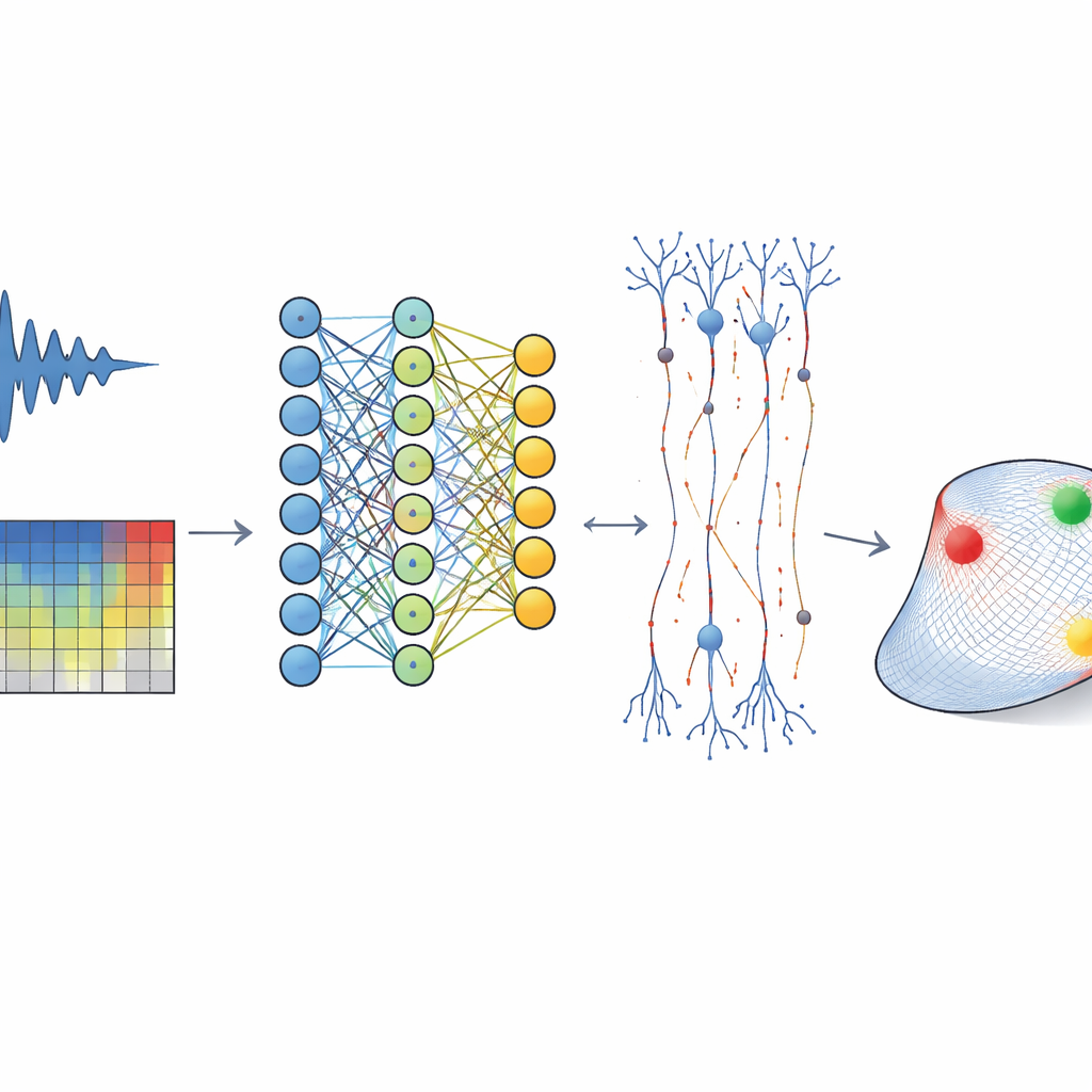
The researchers recorded electrical activity from thousands of individual neurons in the auditory cortex of awake ferrets while the animals listened to a vast library of natural sounds: snippets of speech, music, environmental noises, and animal calls. Instead of using simple tones, the team chose this rich sound diet to better match the complexity of everyday hearing. They converted each sound into a spectrogram, a time–frequency picture of how energy is distributed across pitches over time, and then trained a convolutional neural network (CNN) to predict, millisecond by millisecond, how each neuron would fire. As in other sensory areas, this deep network outperformed classic linear models that assume each neuron listens through a single fixed “filter.”

Flattening a deep network into a simple sound space

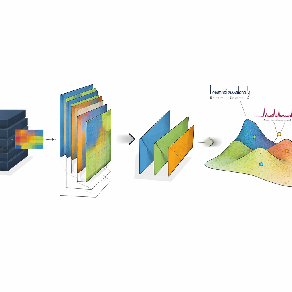
High-performing CNNs are often criticized as black boxes: they match data but are hard to interpret. To tackle this, the authors developed a way to “flatten” the deep model into a simple, low-dimensional sound space for each neuron. First, they calculated a dynamic receptive field at every moment in time by asking how a tiny change in the input spectrogram would alter the CNN’s output for that neuron. This produced a large collection of moment-by-moment filters capturing how the model’s prediction depends on recent sound. They then used a statistical technique to summarize these many filters as a handful of principal components—typically only 3 to 13—which together define a neuron’s tuning subspace: the small set of sound patterns that actually influence its activity.

Reading out nonlinear responses in this shared space

Once sounds were projected into a neuron’s tuning subspace, the team measured how firing rate varied across positions in this reduced space, forming what they call subspace receptive fields. These surfaces were often curved and multi-peaked, revealing rich nonlinear behavior that simple models miss: some neurons responded strongly to several distinct sound patterns, others to both positive and negative deviations along a dimension, and many showed sharp pockets of sensitivity surrounded by zones of suppression. Crucially, a new model that used only the subspace projection plus a modest nonlinear readout predicted neural activity almost as well as the original CNN, capturing over 95% of its explained variance. This shows that the deep model’s complexity can be distilled into a compact, interpretable description of what each neuron is “listening for.”

How neighbors share and divide the work

Because the recordings spanned many neurons along the same cortical column, the authors could ask how local populations share the job of encoding sound. They found that neurons at a given site largely inhabit the same tuning subspace: their preferred sound patterns draw from a common low-dimensional set of features, likely reflecting shared input from earlier stages. Yet within that shared space, each neuron’s high-activity region occupies only a small patch, and these patches overlap no more than if they were scattered at random. In other words, nearby neurons listen to similar kinds of sounds but respond strongly to different specific combinations, forming a sparse tiling of the space. This arrangement explains why neighboring cells often fire very differently to the same natural sound, despite sharing broad preferences such as best frequency.

Different cell types, different roles

The team also leveraged differences in spike shape and recording depth to separate putative excitatory and inhibitory neurons and to assign them to cortical layers. Inhibitory cells, identified by their narrow spikes, tended to have broader subspace receptive fields, meaning they respond across larger regions of the shared sound space. Their nonlinear tuning was more likely to form bowl-like shapes in which strong responses occur for large fluctuations in either direction along a dimension. Excitatory cells, by contrast, more often showed peaked, hill-like tuning confined to a narrower range of inputs. Together, these patterns support a picture in which broadly tuned inhibitory neurons help sculpt a sparse, selective code among their more narrowly tuned excitatory neighbors, with the balance of these effects changing across cortical layers.

Why this framework matters

This work demonstrates that deep neural networks trained directly on brain data can be translated into intuitive maps of what sensory neurons encode and how local circuits are organized. By showing that a small set of shared sound features underlies the responses of many nearby neurons, while individual cells carve out distinct niches within that space, the study provides a concrete framework for thinking about sparse coding, gain control, and invariance in auditory cortex. More broadly, the same “flattening” strategy can be applied in other brain areas, turning powerful but opaque deep-learning models into clear hypotheses about the computations that natural neural circuits perform.

Citation: Wingert, J.C., Parida, S., Norman-Haignere, S.V. et al. Convolutional neural network models describe the encoding subspace of local circuits in auditory cortex. Nat Neurosci 29, 876–887 (2026). https://doi.org/10.1038/s41593-026-02216-0

Keywords: auditory cortex, convolutional neural networks, neural encoding, sparse coding, sensory subspace