Comparative evaluation of several models for forecasting hourly electricity use in a steel plant

Why predicting a factory’s power use matters

Steel plants are among the hungriest users of electricity on the planet, and every unexpected spike in power demand shows up directly on their monthly bill. If managers can see those spikes coming, even just a few hours ahead, they can shift production schedules, avoid costly penalties from the grid, and cut their carbon footprint. This study looks at how three modern data-driven tools stack up when asked a seemingly simple but economically crucial question: how much electricity will a steel plant use in the next hour?

Following the rhythm of a busy steelworks

Inside an integrated steel plant, electricity use rises and falls with the rhythm of furnaces, rolling mills, and maintenance breaks. Hour by hour, demand reflects shift changes, workdays versus weekends, and the timing of energy-hungry steps like heating and rolling. The authors use a full year of real operating data from a large Chinese steel enterprise, giving them 8,760 hourly data points that trace these daily and weekly cycles. Their goal is to turn this historical record into a reliable short-term forecasting tool that plant managers could use to plan production and negotiate better electricity contracts.

Cleaning imperfect data before making predictions

Real-world factory data are messy: sensors fail, meters misread, and occasional extreme operating conditions create outliers. Before building any forecasting models, the researchers therefore clean the data in a careful but simple way. They first flag suspicious readings that sit far outside the typical range of values using a three-sigma statistical rule. Rather than trusting those extreme points, they treat them as missing and fill the gaps by drawing straight lines between the surrounding normal readings along the time axis. Finally, they split the cleaned year of data into three chronological blocks—one to train the models, one to fine-tune them, and the last part of the year to test how well they really perform on unseen future hours.

Three different ways to learn from the past

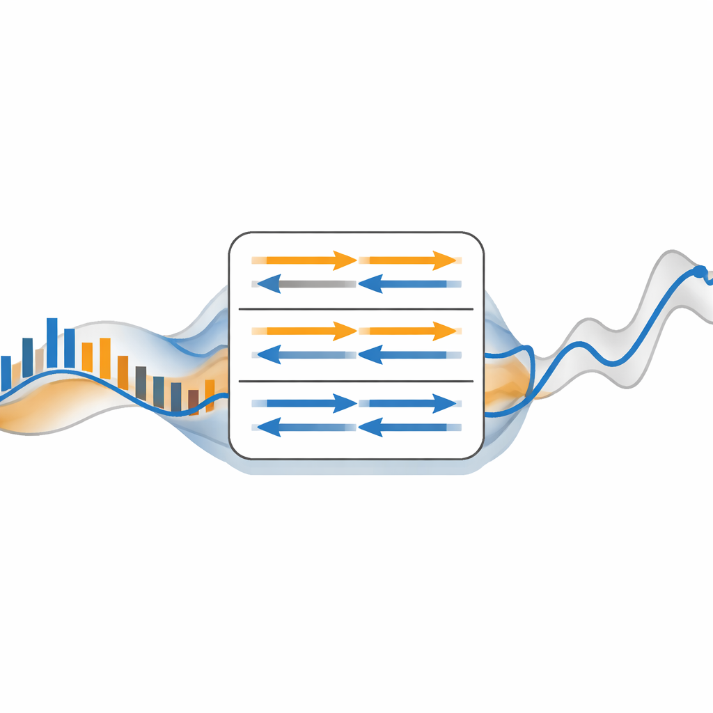
On this common foundation, the study compares three representative forecasting engines. The first, called XGBoost, builds many small decision trees that together learn how past hourly loads relate to the next value. The other two are deep-learning approaches that treat the load record as a sequence in time. A standard Long Short-Term Memory (LSTM) network learns how information flows from past to future, storing patterns in an internal “memory” as it scans through the previous 24 hours. Its cousin, the Bidirectional LSTM (BiLSTM), goes one step further: it processes each 24-hour window in both directions, effectively looking at how recent hours relate not only to what came before but also to what comes immediately after within the window. All three models are asked to look back over the previous day and predict the plant’s consumption for the next hour.

Which model tracks the ups and downs best?

To judge performance, the authors use standard error measures that capture both the size of the typical mistake and how large that mistake is compared with the true value, which is especially important when the plant is running at low load. All three models manage to reproduce the familiar daily rise and fall of electricity demand, but their accuracy differs. The BiLSTM model delivers the lowest errors across the board, closely tracing the real peaks and valleys in the final month of data. XGBoost follows the overall trend well and is comparatively robust, though it tends to miss sharp spikes. The one-directional LSTM improves slightly on XGBoost in some absolute error measures but stumbles more often when the load is low, giving it higher relative error and a more obviously lagging fit during certain peak and valley periods.

What this means for steel plants and beyond

For a lay reader, the headline result is straightforward: when it comes to predicting a steel plant’s electricity use hour by hour, a bidirectional deep-learning model that reads the recent past in both directions beats both a popular tree-based machine-learning method and a simpler recurrent neural network. This advantage translates directly into better cost control and smoother operation, because managers can trust the forecasts that guide their scheduling and demand-response decisions. At the same time, the study shows that careful but uncomplicated data cleaning and a fair, unified testing setup are just as important as the choice of model. While the work focuses on one plant and a single year of data, it suggests that similar approaches could help many energy-intensive factories tame their power bills and shrink their emissions.

Citation: Gu, F., Zhao, Y. Comparative evaluation of several models for forecasting hourly electricity use in a steel plant. Sci Rep 16, 13123 (2026). https://doi.org/10.1038/s41598-026-43868-z

Keywords: steel plant electricity, short-term load forecasting, deep learning energy, industrial energy management, BiLSTM forecasting