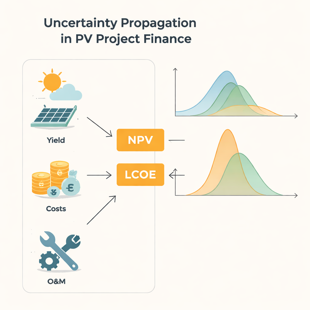
Anyone financing a solar power plant is essentially making a 20‑ to 30‑year bet on sunshine, prices, and costs. But all of these ingredients are uncertain: weather fluctuates, equipment wears out in unpredictable ways, and future electricity prices are never guaranteed. This paper asks a practical question at the heart of the clean‑energy transition: how does that uncertainty in the inputs of a financial spreadsheet really affect the bottom line for a photovoltaic (PV) project, and are today’s common shortcuts good enough?
From simple guesses to full uncertainty pictures
Traditional project evaluations often reduce uncertainty to a few rough “what‑if” scenarios or to compact summary numbers like averages and standard deviations. A standard engineering guide known as GUM provides formulas that approximate how input variability ripples through to outputs such as the net present value (NPV) and the levelized cost of electricity (LCOE). These shortcuts treat the model as almost linear and usually assume that the outputs behave like neat bell curves. That works when fluctuations are small and the equations are gentle. But solar power is driven by weather and failures that can be highly erratic, and long project lifetimes mean the same uncertain processes repeat year after year. In such cases, the familiar formulas can quietly break down, especially when the model includes nonlinear pieces like ratios.
A faster route to full probability distributions Figure 1.
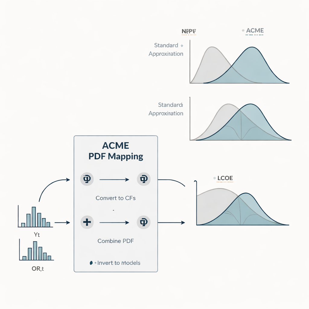
To tackle this, the authors introduce a new method called ACME (Accelerating Conversion of Mapping Equations). Instead of tracking just averages and spreads, ACME follows the entire probability distributions from input variables to financial outputs. It treats yearly energy yield and repair‑related operation and maintenance costs as random quantities with shapes guided by field data: yields follow a flexible distribution that can mimic near‑Gaussian or strongly skewed behavior, while repair costs follow an exponential pattern with many small events and a few large ones. ACME works by exploiting the mathematical fact that sums of independent random contributions can be handled efficiently in Fourier space, using so‑called characteristic functions. By switching between this representation and more familiar probability curves, the method collapses what would be huge, high‑dimensional integrals into a few one‑dimensional ones. The result is a numerically light way to obtain full distributions for NPV and LCOE without resorting to massive Monte Carlo simulations.
Testing three worlds of uncertainty
The study compares ACME with the standard GUM approximation in a case study of a typical rooftop‑scale PV system. The authors construct three scenarios that all share the same expected energy production and cost levels but differ in how uncertain the yearly yield is. In the “O” scenario, yield is almost fixed and only repair costs fluctuate. The “YO” scenario represents moderate yield variability comparable to assumptions in many current studies. The “wYO” scenario pushes yield variability to an extreme, mimicking a future with highly volatile climate or poorly known long‑term conditions. Across these scenarios, the team computes not just mean NPV and LCOE, but also their standard deviations, “P90” values that investors use as conservative benchmarks, the probability that NPV is positive, and how these quantities change with project lifetime from 1 to 30 years.
What happens to risk and return Figure 2.
Several patterns emerge. Because NPV is linear in the chosen uncertain inputs, its average value depends mainly on expected yields and costs, not on how uncertain they are, while its spread grows with both project lifetime and input variability. LCOE behaves differently: larger yield uncertainty raises the expected cost per kilowatt‑hour, especially for short lifetimes, and its uncertainty actually shrinks as the project runs longer. For mild uncertainties and longer lifetimes, the standard approximation tracks ACME closely. But when yield uncertainty is large and enters the LCOE formula in a nonlinear way, the shortcut systematically underestimates both the mean LCOE and its variability, and it can misrepresent the shape of the distribution, which often departs strongly from a bell curve. The analysis of cumulative distributions shows that these mismatches can distort widely used risk measures such as P90 values and the perceived probability of hitting a given cost band.
What this means for investors and planners
For a non‑specialist, the message is straightforward: the amount and shape of uncertainty in solar yield and repair costs can noticeably change conclusions about a project’s risk and competitiveness, even when long‑run averages stay the same. Simple formulas that assume small fluctuations and bell‑shaped behavior may be adequate for stable conditions, long lifetimes, or nearly linear models, but they can give overly optimistic pictures when uncertainty is large or enters through ratios like LCOE. ACME offers a practical way to obtain a full picture of possible financial outcomes, including skewed or heavy‑tailed cases, at a computational cost far below brute‑force simulation. As PV expands and climate and market volatility grow, such richer uncertainty modeling can help investors, banks, and policymakers judge solar projects more realistically and design support schemes that reflect not only expected returns but also the range of risks.
Citation: Wieland, S., Gürsal, U. Uncertainty propagation in financial models of photovoltaic systems.
Sci Rep16, 5004 (2026). https://doi.org/10.1038/s41598-026-38053-1
Keywords: photovoltaic finance, uncertainty propagation, solar investment risk, levelized cost of electricity, net present value